Technology and Digital TransformationData Analytics
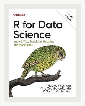
Summary of “R for Data Science: Import, Tidy, Transform, Visualize, and Model Data”
Authors: Hadley Wickham, Garrett Grolemund
Publication Year: 2016
Category: Data Analytics
1. Introduction: The Basics of R and Data Science
Action: Set up R and RStudio on your computer.
– The book opens by emphasizing the importance of R and RStudio in modern data science. It guides beginners through installing and configuring the software and packages that are essential for data science workflows, such as tidyverse.
Concrete Example: “To install tidyverse, you simply use the command install.packages('tidyverse') in your R console.”
2. Data Importing: Getting Data into R
Action: Use the read_csv() function to import CSV files.
– One of the first key sections focuses on importing data into R from various sources including CSV files, Excel spreadsheets, and databases.
– The readr package is highlighted for its efficiency in reading different data formats into R.
Concrete Example: “You can read a CSV file into R using data <- read_csv('path/to/your/file.csv'). This loads your CSV data into a dataframe named data.”
3. Data Tidying: Structuring Your Data
Action: Use gather() and spread() functions to reshape data.
– The book dives into the principles of tidy data, advocating that each variable should have its own column, each observation its own row, and each type of observational unit its own table.
– Functions from the tidyr package like gather() (to convert wide data into long data) and spread() (to convert long data into wide data) are crucial.
Concrete Example: “To convert your data from wide to long format, use data_long <- gather(data, key = 'variable', value = 'value', -identifier_column).”
4. Data Transformation: Using dplyr for Data Manipulation
Action: Use filter(), select(), mutate(), summarize(), and arrange() functions to manipulate data.
– The book emphasizes the dplyr package for data manipulation tasks such as filtering rows, selecting columns, creating new variables, and summarizing data.
– Each function is broken down with clear examples.
Concrete Example:
– “To filter rows where a variable x is greater than 100: filtered_data <- filter(data, x > 100).”
– “To create a new variable: data <- mutate(data, new_variable = variable1 / variable2).”
5. Exploratory Data Analysis (EDA): Visualizing Data
Action: Create visualizations using ggplot2.
– Visualization is crucial in EDA, and the authors present ggplot2 as the main tool for creating comprehensive visualizations.
– The book covers basic to advanced plots, explaining the layering system of ggplot2 and its syntax.
Concrete Example:
– “To create a scatter plot: ggplot(data, aes(x = variable1, y = variable2)) + geom_point().”
– “For a histogram: ggplot(data, aes(x = variable)) + geom_histogram(binwidth = 10).”
6. Data Modeling: Understanding and Applying Models
Action: Use lm() for linear modeling.
– The book introduces statistical modeling as a method to understand relationships between variables. It covers linear models, generalized linear models, and other types of predictive analytics.
– Emphasis on learning the basics of modeling starting with linear models using functions such as lm().
Concrete Example: “To fit a linear model: model <- lm(outcome ~ predictor, data = dataset).”
7. Communicating Results: Sharing Your Work
Action: Use R Markdown to create reports.
– Communicating data science results is emphasized as crucial, and the book highlights the use of R Markdown for creating dynamic documents that integrate code, its output, and narrative text.
– This section includes how to generate HTML, PDF, and Word documents from R Markdown files.
Concrete Example: “To create a markdown document, initialize with File -> New File -> R Markdown…, write your narrative and R code chunks, then click Knit to render.”
8. Workflow: Managing Data Science Projects
Action: Utilize version control with Git and GitHub.
– The book underscores the importance of a robust workflow for data science projects. Topics include organizing project directories, using version control with Git and GitHub, and documenting your work for reproducibility.
Concrete Example: “To track changes with Git, initialize a repository in your project folder using git init and commit changes with git commit -m 'your commit message'.”
Conclusion: Becoming a Successful Data Scientist
Action: Engage in continuous learning and practice.
– The authors stress the need for continuous learning and practice. They encourage participation in data science communities, attending workshops, and staying updated with the latest trends and tools.
Concrete Example: “Enroll in online courses such as those offered by Coursera or DataCamp, and participate in forums like RStudio Community or Stack Overflow to learn and share knowledge.”
Closing Thoughts
“R for Data Science” is an invaluable resource that covers a comprehensive range of topics essential for any data scientist. By following the concrete examples and actions provided throughout the book, readers can effectively import, tidy, transform, visualize, and model their data using R. The book’s structure and practical examples ensure that both novice and experienced data analysts can benefit from its teachings.
